
The US spends over $4 trillion per year on healthcare, which is largely conducted by private providers and reimbursed by insurers. Overbilling, waste, and fraud are major concerns in the healthcare system and are estimated by the US Federal Bureau of Investigation to account for 3% to 10% of overall spending. Provider fraud occurs when healthcare providers misreport their claims to receive higher payments. In this work, I use large-scale claims data from Medicare, the US federal health insurance program for elderly adults and the disabled, to perform an exploratory data analysis. My goal is to identify patterns consistent with fraud or overbilling and understand characteristics associated with high suspiciousness of fraud. My proposed approach for fraud detection is supervised and involves developing a broad range of classifiers on labeled training data to help identify potential providers who might overbill insurers. I also provide reasoning and interpretable insights into the potentially suspicious behavior of flagged providers by analyzing important features. Additionally, I apply SMOTE techniques to handle imbalanced data and improve 1-fold lift recall for the minority/fraud class. The results can be used to guide investigations and auditing of suspicious providers for both public and private health insurance systems.
Healthcare Provider Fraud overview
Healthcare fraud and abuse take many forms. Some of the most common types that providers deceive insurers through claims procedures are listed below:
- Phantom Billing. Providers billing for services not provided.
- Unnecessary Services. Providers administering (more) tests and treatments that are not medically necessary.
- Upcoding. Providers administering more expensive tests and equipments.
- Multiple-billing. Providers multiple-billing for services rendered.
- Unbundling. Providers unbundling or billing separately for laboratory tests to get higher reimbursements.
- False price reporting. Providers charging more than peers for the same services.
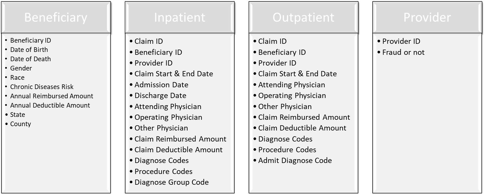
Medicare claims dataset
The dataset in this project comes from Kaggle’s website - Healthcare Provider Fraud Dection Analysis by Rohit Anand Gupta. The dataset consists of four sub-datasets, as listed below.
Workflow

Data Preporcessing
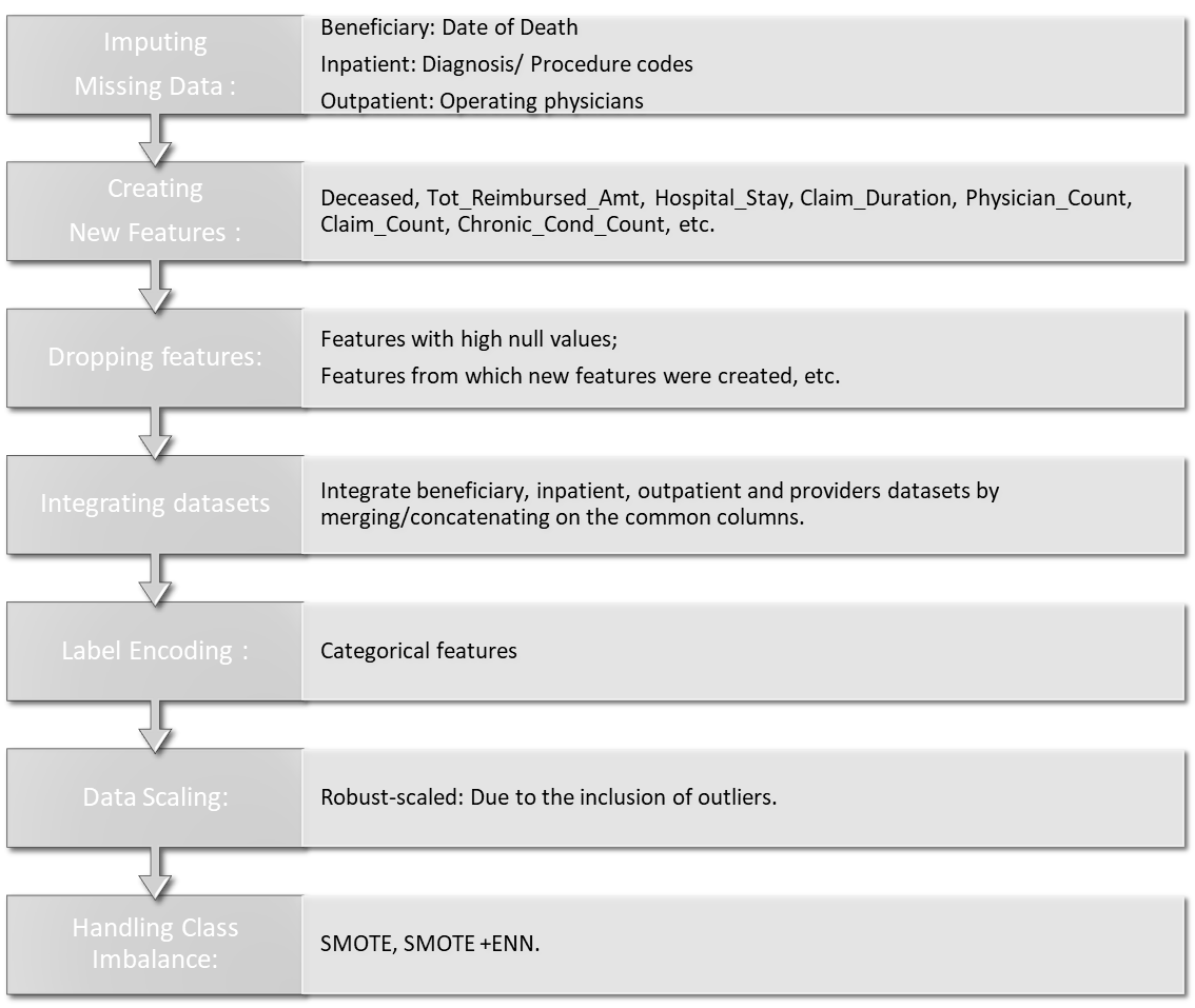
Before discussing the extensive data analysis performed on the claims data, I would like to explain how the data was preprocessed. First, I handled missing values in the data by imputing them accordingly. I also enriched the data by creating new features. For example, in the beneficiaries dataset, the date of death was missing if a patient was alive. I created two new features: ‘if-alive’ and ‘Age’ using the date of birth and death.
Next, I label-encoded categorical data and scaled numerical data for uniform and efficient preprocessing. Here, I used RobustScaler to scale features because it is robust to outliers. The outliers in the data were kept, as they could provide important fraud indicator information and sometimes represent actual fraud transactions were being committed sometim.
Another important preprocessing step was resampling the imbalanced data to make class ratio to 1:1. Data imbalance is a typical scenario in many business problems like fraud detection, spam filtering, rare disease discovery, hardware fault detection, etc. In general, the minority/positive class is the main concern and is aimed to achieve the best results. If imbalanced data is not treated beforehand, most predictions will correspond to the majority class and treat minority class features as noise in the data and ignore them. This will result in high bias in the classifier model and degrade the model performance. Resampling data is one of the most common approaches to deal with an imbalanced dataset, including undersampling and oversampling. Here, I used two resampling techniques: 1) SMOTE, which randomly oversamples data by choosing one of K instances to interpolate new synthetic instances; and 2) SMOTE+ENN, which is a hybrid technique. ENN is an undersampling technique that removes the nearest neighbors of each majority class instance. Integrating ENN with SMOTE can clean overlapping data points for each class distributed in sample space and optimize the performance of classifier models while avoiding overfitting.
Exploratory Data Analysis
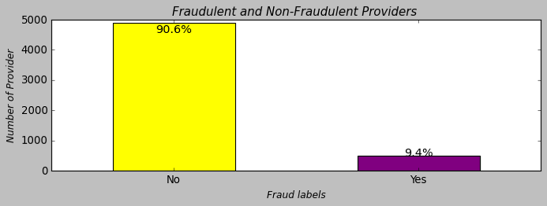
1. Class Labels
Let’s take a look at the provider class dataset. It is an imbalanced dataset where the target variable, “Potential Fraud,” has 90.6% of providers not fraudulent and 9.6% of providers fraudulent. The accuracy metric is not preferable to evlauate the model performance for imbalanced classes. At the model evlaluation section, we will use metrics like precision, recall, F1-score rather than the accuracy metric to evaluate the performance of the classifiers.
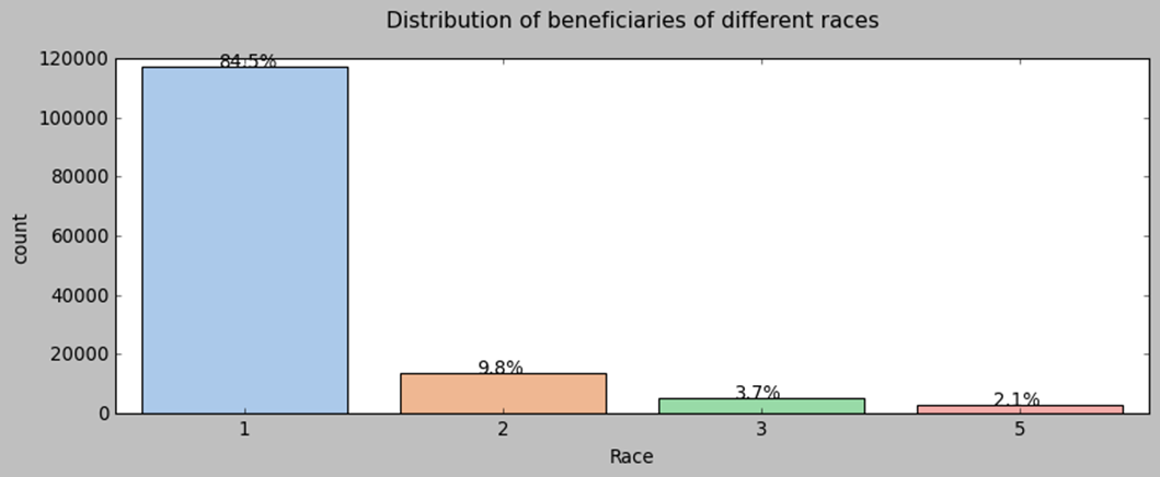
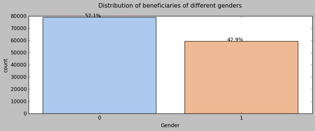
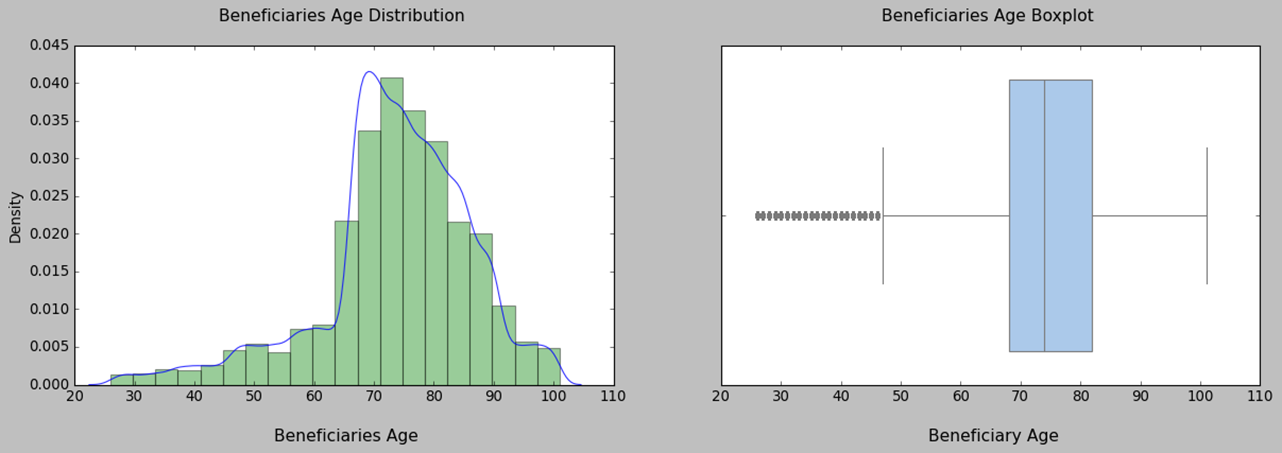
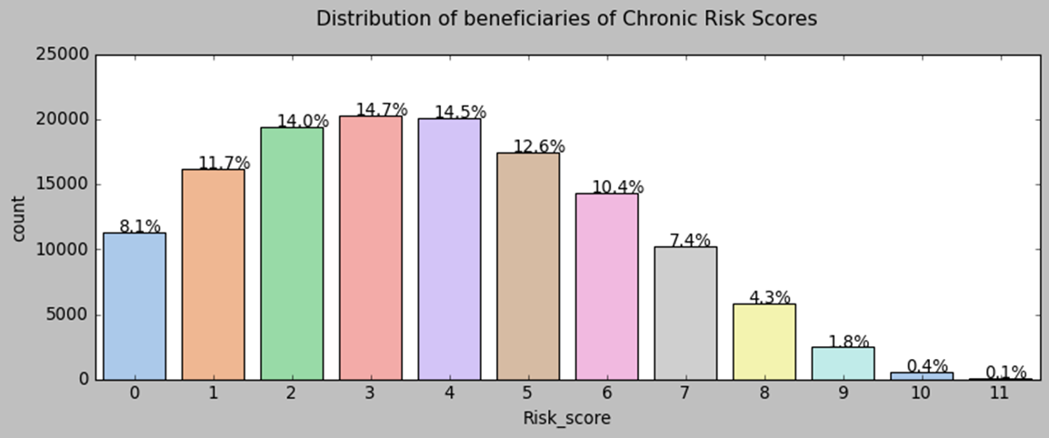
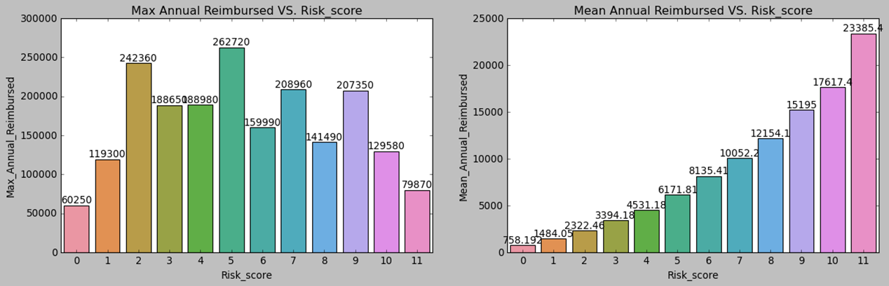
2. Beneficiary Basic Information Study
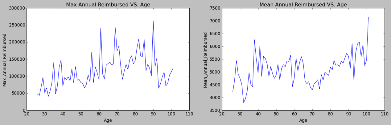
Before we proceed, let’s take a look at our patients. We notice that the majority of our beneficiaries belong to race 1. The percentage of gender 0 is larger than that of gender 1. Fifty percent of beneficiaries fall between the ages of 68 and 82 years old, with some outliers below 47 who are disabled. The chronic disease risk scores display a bell-like shape with a slight right tail. There is a positive relationship between the mean annual reimbursement amount and the chronic disease risk scores of beneficiaries.
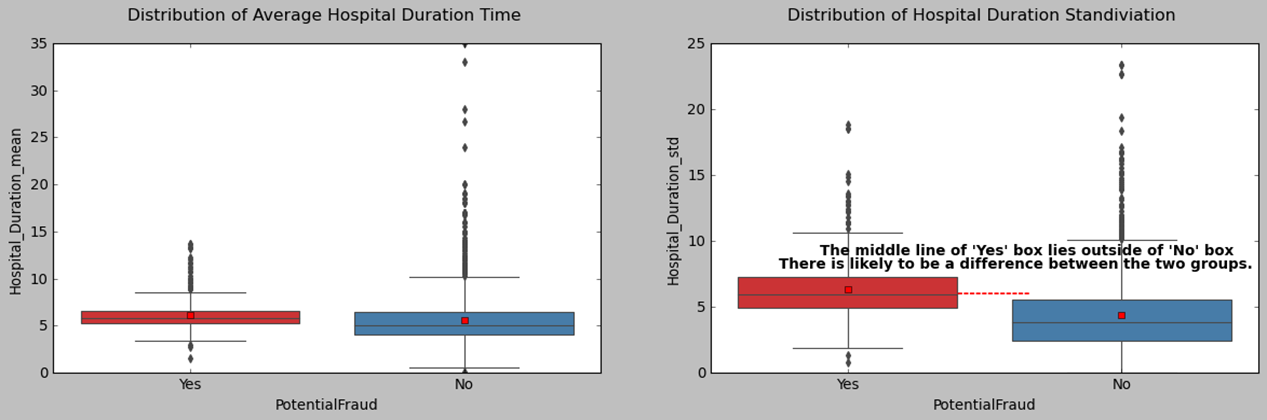
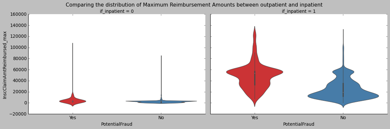
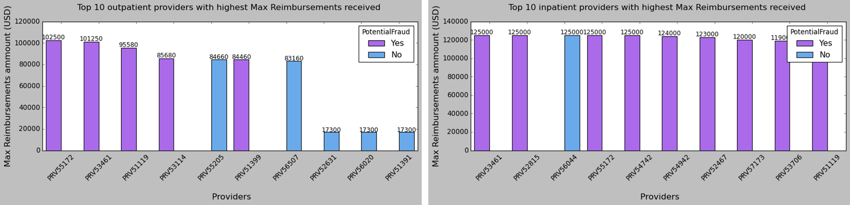
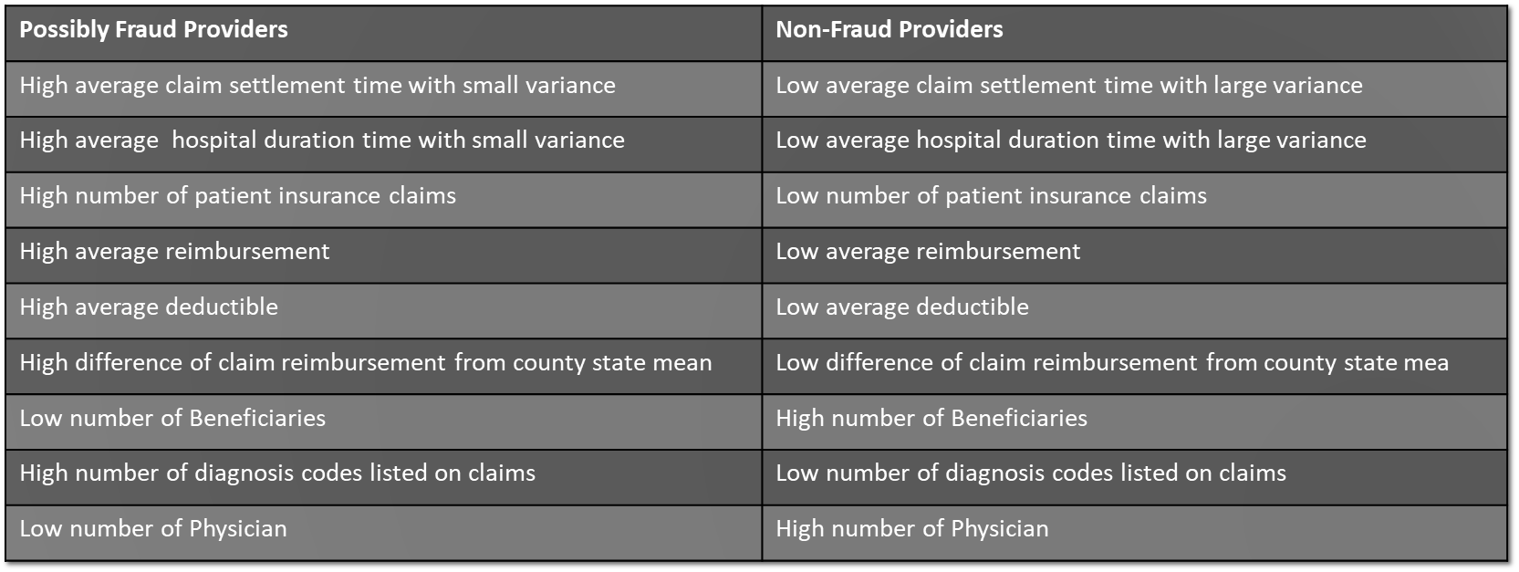
3. fraud VS. Non-fraud Providers Study
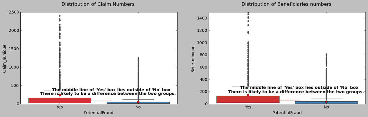
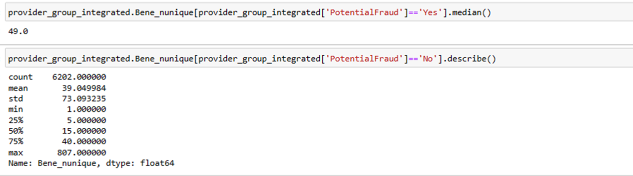
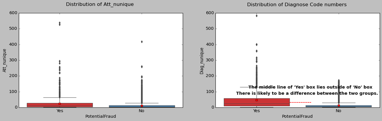
Now, let’s explore the characteristics of fraudulent providers. We know that if the median line of a box plot lies outside the box of a comparison box plot, then there is likely to be a difference between the two groups. When comparing the box plots of characteristics, like claim numbers, beneficiary numbers, diagnose code numbers, and hospital duration variation, we find that there are obvious differences between fraudulent and non-fraudulent providers.
Data Modeling
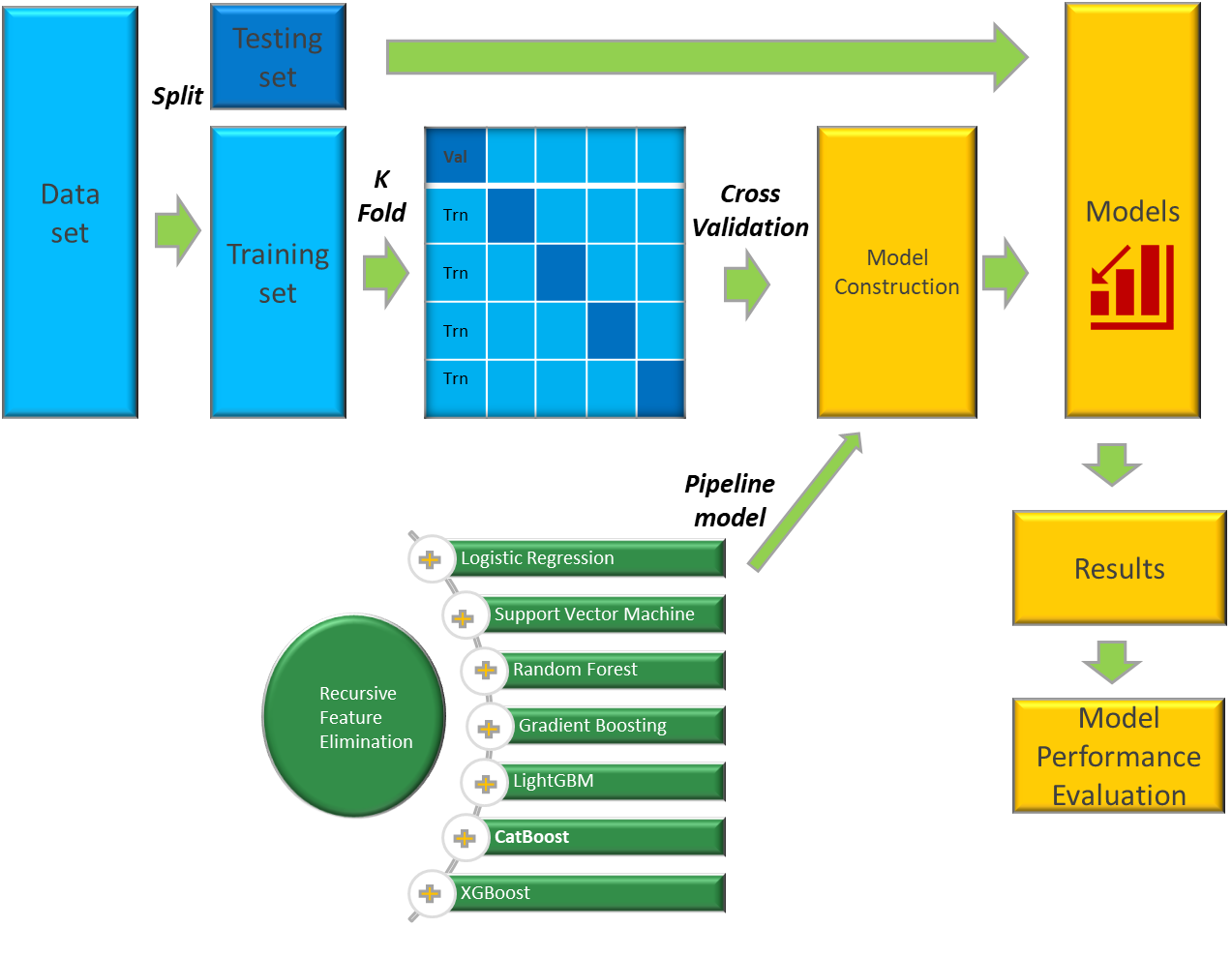
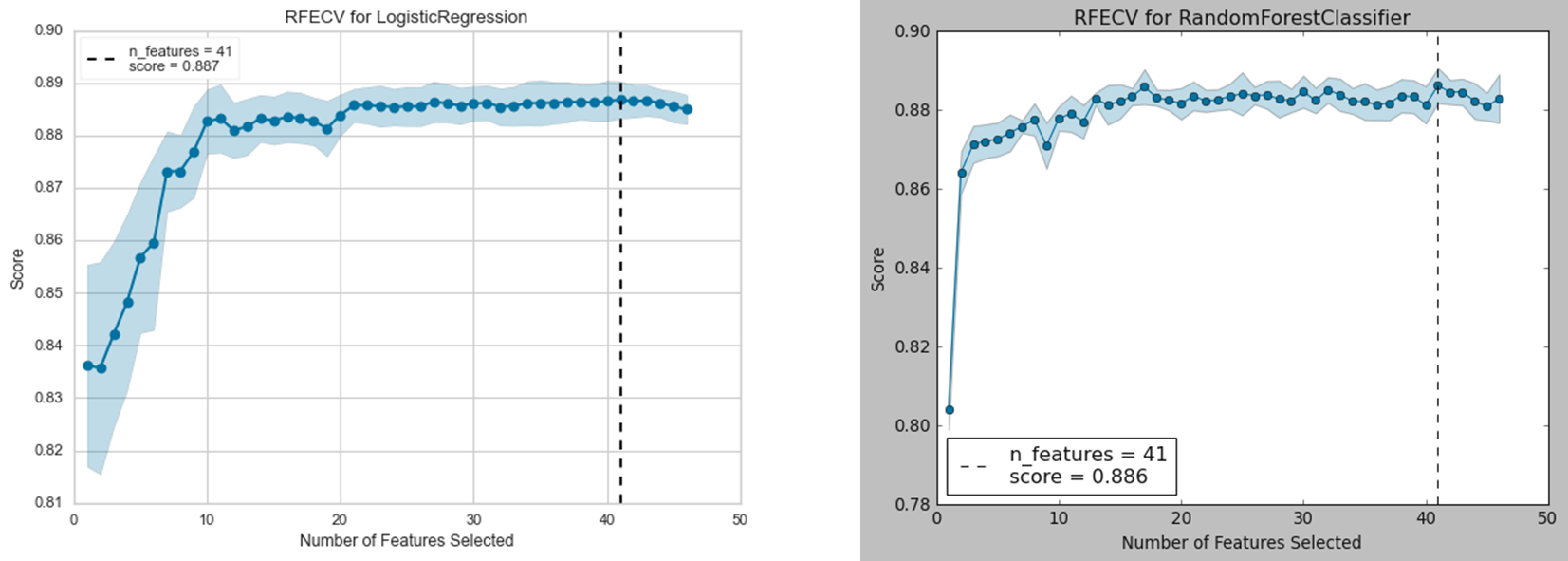
1. Feature Selection
In this section, I will pipleline classifiers and feature selection method to build the base algorithms. I choose RFE method for feature selection, and tune the hyperparameters of RFE to obtian the best number of features, as showed in the below, the number 41 is the best number of features for both logistic regression and random forest algorithms.
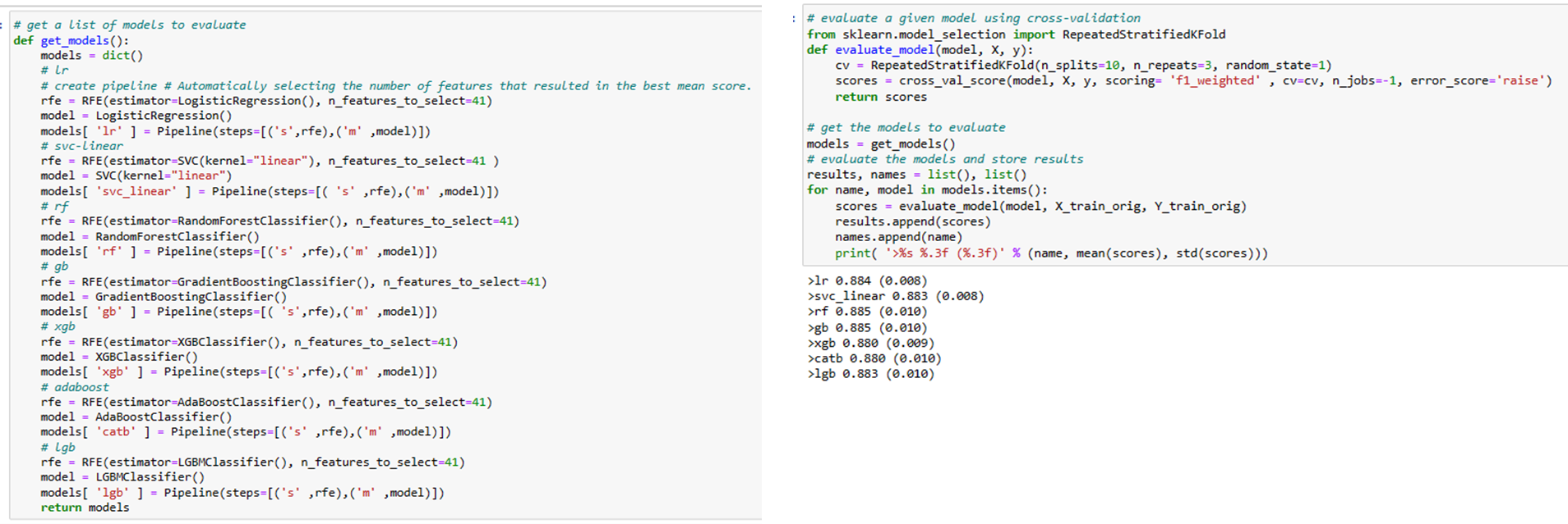
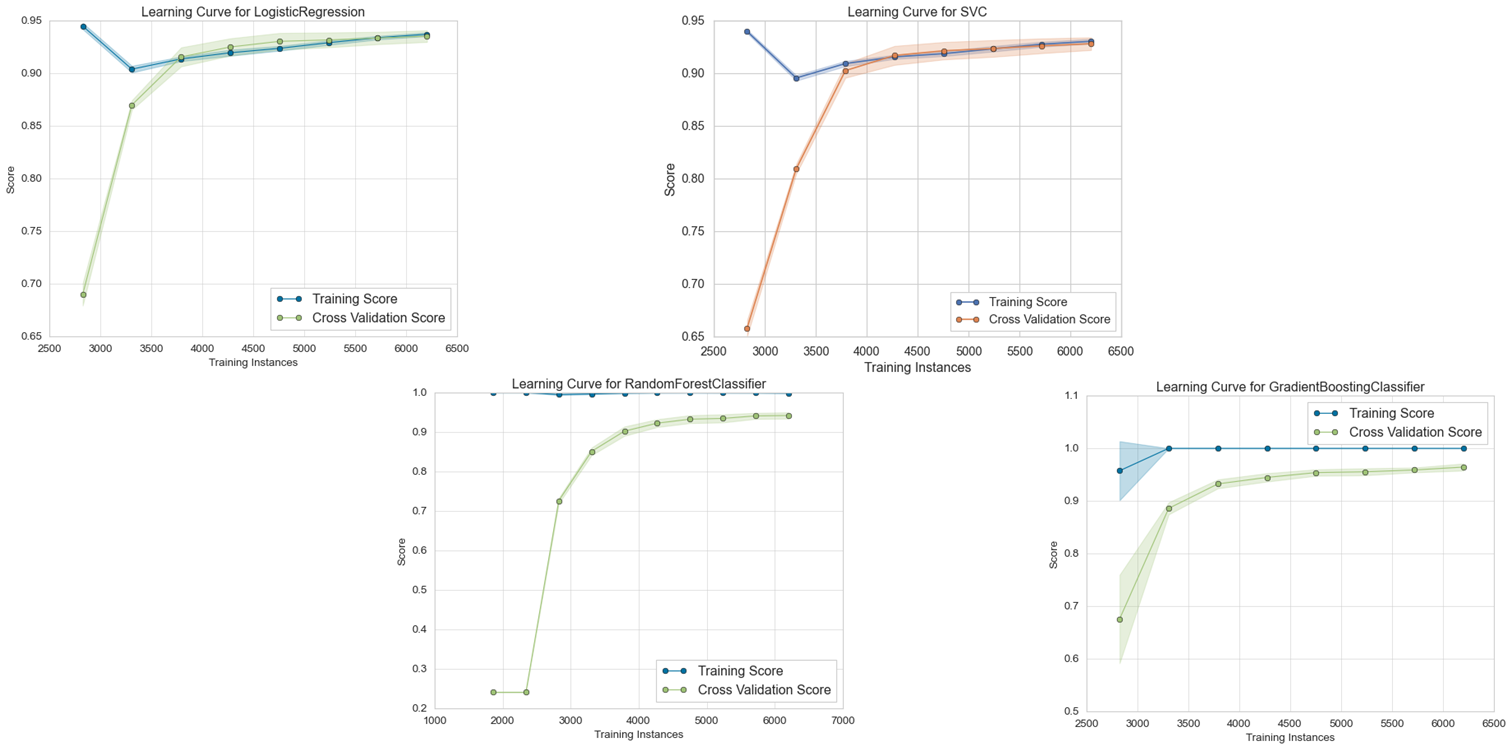
2. Explore Base Algorithm
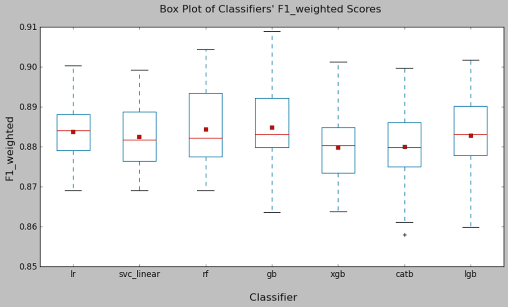
3. Base Algorithm comparison
Logistic Regression, Support Vector Machine, and Random Forest classifiers generally perform well. While the mean performance of the Gradient Boosting classifier appears good, its F1_weighted score has a relatively larger variance compared to the others. This may result in less stable results.
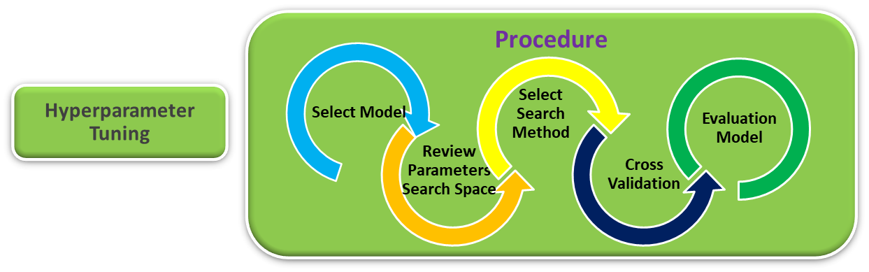
Optimization Models
1. Tune Hyperparameters
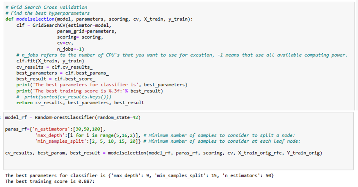
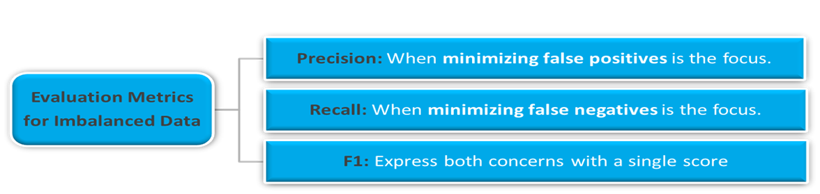
3. Evaluation Metrics for Imbalanced Data
A comparative analysis was performed on the dataset using four classifier models: Logistic Regression, Random Forest, Linear Support Vector Machine, and Gradient Boosting. As discussed earlier, we will ignore the accuracy metric to evaluate the performance of the classifiers on this imbalanced dataset. Here, we are more interested in identifying potential fraudulent providers. Therefore, we will focus on metrics such as precision, recall, and F1-score to understand the performance of the classifiers in correctly determining which providers will commit fraud in the
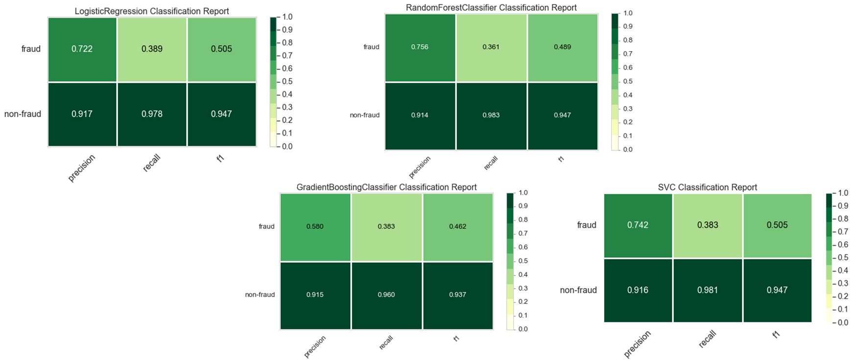
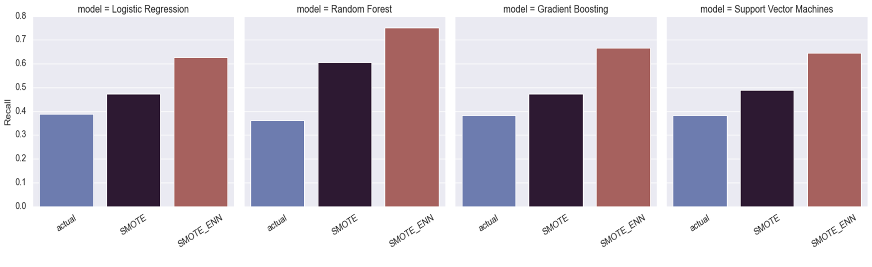
4. Maximize Minority’s Recall Scores
From the above, it can be seen that all 4 classifier models were not able to generalize well on the minority class compared to the majority class. To minimize fraudulent providers incorrectly classified as non-faudulent providers (False Negative), we can use SMOTE related technolege to imporve recall scores of the minority class. As shown in below, after resampling, a clear surge in Recall is seen on the test data.
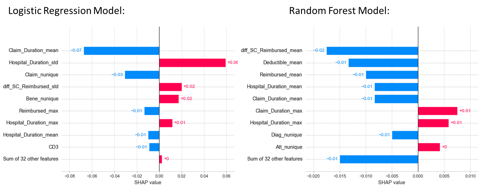
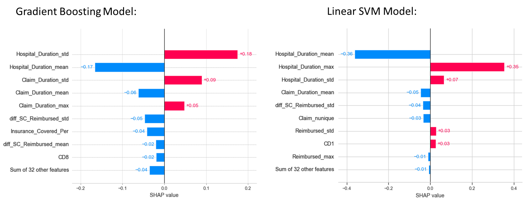
5. Feature Importances
Machine Learning models are often black boxes, making their interpretation difficult. SHAP values (SHapley Additive exPlanations) is one method used to explain how each feature affects the model. The following plots show the main features affecting the prediction of the observations and the magnitude of the SHAP value for each feature. Here, I used shap__value[0], the SHAP values for class 0. The SHAP values for class 1 are symmetrical to them.
Conclusion
The souce code used to create this blog can be found here.