
In this post, I will investigate movies datasets randomly sampled from Rotten Tomatos and IMDB. The purpose of the project is to identify which factors and attributes make movies popular, and develop models to predict audience responses for new movies.
Load packages.
library(tidyverse)
library(dlookr)
library(gridExtra)
library(corrplot)
library(caTools)
library(caret)
library(mlbench)
library("gbm")
library(Metrics)
Load the dataset and take a quick look.
load("movies.RData")
head(movies,2)
# A tibble: 2 × 32
title title_type genre runtime mpaa_rating studio thtr_rel_year thtr_rel_month thtr_rel_day dvd_rel_year dvd_rel_month dvd_rel_day imdb_rating
<chr> <fct> <fct> <dbl> <fct> <fct> <dbl> <dbl> <dbl> <dbl> <dbl> <dbl> <dbl>
1 Filly Brown Feature F… Drama 80 R Indom… 2013 4 19 2013 7 30 5.5
2 The Dish Feature F… Drama 101 PG-13 Warne… 2001 3 14 2001 8 28 7.3
# ℹ 19 more variables: imdb_num_votes <int>, critics_rating <fct>, critics_score <dbl>, audience_rating <fct>, audience_score <dbl>,
# best_pic_nom <fct>, best_pic_win <fct>, best_actor_win <fct>, best_actress_win <fct>, best_dir_win <fct>, top200_box <fct>, director <chr>,
# actor1 <chr>, actor2 <chr>, actor3 <chr>, actor4 <chr>, actor5 <chr>, imdb_url <chr>, rt_url <chr>The data set is comprised of 651 randomly sampled movies produced and released before 2016, Each record in the database describes characteristics of a movie.Some of these variables are only there for informational purposes and do not make any sense to include in a statistical analysis, For example information in the the actor1 through actor5 variables was used to determine whether the movie casts an actor or actress who won a best actor or actress Oscar. We select and create some new variables that might be meaningful to identify the popularity of movies.
-
title_type: Type of movie (Documentary, Feature Film, TV Movie)
-
genre: Genre of movie (Action & Adventure, Comedy, Documentary, Drama, Horror, Mystery & Suspense, Other)
-
runtime: Runtime of movie (in minutes)
-
mpaa_rating: MPAA rating of the movie (G, PG, PG-13, R, Unrated)
-
imdb_rating: Rating on IMDB
-
imdb_num_votes: Number of votes on IMDB
-
critics_rating: Categorical variable for critics rating on Rotten Tomatoes (Certified Fresh, Fresh, Rotten)
-
critics_score: Critics score on Rotten Tomatoes
-
audience_rating: Categorical variable for audience rating on Rotten Tomatoes (Spilled, Upright)
-
audience_score: Audience score on Rotten Tomatoes
-
best_pic_win: Whether or not the movie won a best picture Oscar (no, yes)
-
best_actor_win: Whether or not one of the main actors in the movie ever won an Oscar (no, yes)
-
best_actress win: Whether or not one of the main actresses in the movie ever won an Oscar (no, yes)
-
best_dir_win: Whether or not the director of the movie ever won an Oscar (no, yes)
-
top200_box: Whether or not the movie is in the Top 200 Box Office list on BoxOfficeMojo (no, yes)
-
oscar_season: New variable, Whether or not the movie is released in theaters during the oscar season.
-
summer_season: New variable, Whether or not the movie is released in theaters during the summer season.
1. Data Preparation
# creating new features
# Column for if movie was released during oscar season
movies <- movies %>%
  mutate(oscar_season = as.factor(ifelse(thtr_rel_month %in% c('10', '11', '12'), 'yes', 'no')))
# Column for if movie was released during summer season
movies <- movies %>%
  mutate(summer_season = as.factor(ifelse(thtr_rel_month %in% c('6', '7', '8'), 'yes', 'no')))

# Extracting meaningful features.
movies_new <- movies %>% select(title_type, genre, runtime, mpaa_rating, imdb_rating, imdb_num_votes, critics_rating, critics_score, audience_rating, audience_score, best_pic_win, best_actor_win, best_actress_win, best_dir_win, top200_box, oscar_season, summer_season)
Let’s check and deal with missing values.
cat("Number of missing value:", sum(is.na(movies_new)), "\n")
plot_na_pareto(movies_new)
Number of missing value: 1 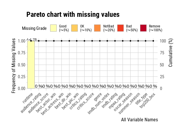
movies_new<-movies_new %>%
  na.omit(runtime)
Split the data sets into a training Dataset and a testing Dataset,
set.seed(101)
sample = sample.split(movies_new$audience_score, SplitRatio = .8)
train = subset(movies_new, sample == TRUE)
test  = subset(movies_new, sample == FALSE)
2. Analyze Data
2.1 Descriptive Statistics
dim(train)
# summarize feature distributions
summary(train)
# Let's also look at the data types of each feature.
sapply(train, class)
title_type genre runtime mpaa_rating imdb_rating imdb_num_votes critics_rating critics_score
Documentary : 44 Drama :255 Min. : 39.0 G : 16 Min. :1.900 Min. : 180 Certified Fresh: 99 Min. : 1.00
Feature Film:473 Comedy : 63 1st Qu.: 92.0 NC-17 : 2 1st Qu.:5.900 1st Qu.: 4375 Fresh :173 1st Qu.: 32.00
TV Movie : 4 Action & Adventure: 47 Median :102.0 PG : 95 Median :6.600 Median : 15025 Rotten :249 Median : 61.00
Documentary : 43 Mean :105.5 PG-13 :104 Mean :6.477 Mean : 56558 Mean : 56.91
Mystery & Suspense: 42 3rd Qu.:115.0 R :266 3rd Qu.:7.300 3rd Qu.: 57251 3rd Qu.: 82.00
Horror : 19 Max. :267.0 Unrated: 38 Max. :9.000 Max. :893008 Max. :100.00
(Other) : 52
audience_rating audience_score best_pic_win best_actor_win best_actress_win best_dir_win top200_box oscar_season summer_season
Spilled:220 Min. :11.00 no :518 no :443 no :469 no :489 no :510 no :373 no :389
Upright:301 1st Qu.:46.00 yes: 3 yes: 78 yes: 52 yes: 32 yes: 11 yes:148 yes:132
Median :65.00
Mean :62.45
3rd Qu.:80.00
Max. :97.00
title_type genre runtime mpaa_rating imdb_rating imdb_num_votes critics_rating critics_score
"factor" "factor" "numeric" "factor" "numeric" "integer" "factor" "numeric"
audience_rating audience_score best_pic_win best_actor_win best_actress_win best_dir_win top200_box oscar_season
"factor" "numeric" "factor" "factor" "factor" "factor" "factor" "factor"
summer_season
"factor" 2.2 Data Visualizations
Correlation between categorical feature and audience score
names <- names(Filter(is.factor,train))
plot_list <- list()

for (name in names) {
  plot <- ggplot(data = train, aes_string(x = name, y = train$audience_score, fill = name)) +
    geom_boxplot(show.legend=FALSE) + xlab(name) + ylab('Audience Score')
  plot_list[[name]] <- plot
}
plot_grob <- arrangeGrob(grobs=plot_list, ncol=3)
grid.arrange(plot_grob)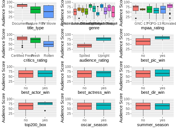
As we know, if median value lines from two different boxplots do not overlap, then there is a statistically significant difference between the medians. Therefore, it looks that best_actor_win, best_actress_win, best_dir_win, top200_box, oscar_season and summer_season do not seem to have much impact on audience_score.
Bar plot of categorical features
plot_list2 <- list()
for (name in names[1:6]) {
  plot <- ggplot(aes_string(x=name), data=train) + geom_bar(aes(y=100*(..count..)/sum(..count..))) + ylab('percentage')  +
    ggtitle(name) + coord_flip()
  plot_list2[[name]] <- plot
}
plot_grob2 <- arrangeGrob(grobs=plot_list2, ncol=2)
grid.arrange(plot_grob2)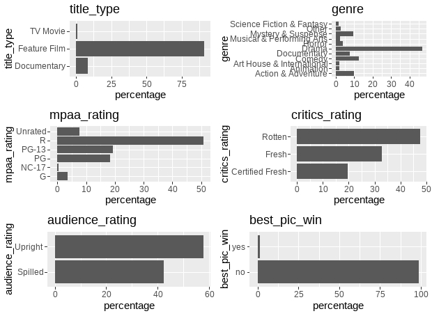
Critics_rating, audience_rating have observations spread out fairly evenly over all categories shows high variability, while “title_type”, “genre”, “mpaa_rating” and “best_pic_win” where most observations are only in one or a handful of categories displays low variability.
Histogram of Numeric attributes
names_n <- names(Filter(is.numeric,train))
hisplot_list <- list()
for (name in names_n) {
  plot <- ggplot(data = train, aes_string(x = name)) +
    geom_histogram(aes(y=100*(..count..)/sum(..count..)), color='black', fill='white') + ylab('percentage') + ggtitle(name)
  hisplot_list[[name]] <- plot
}
hisplot_grob <- arrangeGrob(grobs=hisplot_list, ncol=2)
grid.arrange(hisplot_grob)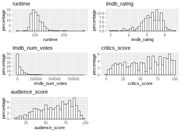
The distribution of attribute imdb_num_votes is right skewed, will be shifted by using The BoxCox transform to reduce the skew and make it more Gaussian
Correlation between numerical attributes
corr.matrix <- cor(train[names_n])
corrplot(corr.matrix, main="\n\nCorrelation Plot of numerical attributes", method="number")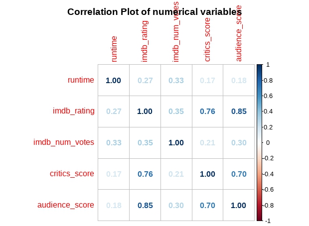
Summary of Ideas
There is a lot of structure in this dataset. We need to think about transforms that we could use later to better expose the structure which in turn may improve modeling accuracy. So far it would be worth trying:
- Feature selection and removing the most correlated attributes.
- standardizing the dataset to reduce the effect of differing scales and distributions.
- Box-Cox transform to see if flattening out some of the distributions improves accuracy.
3. Data transformation
sapply(train[names_n],class)
train$imdb_num_votes <- as.numeric(train$imdb_num_votes)
train_num <- as.data.frame(train[names_n])
# calculate the pre-process parameters from the dataset
preprocessParams <- preProcess(train_num, method=c("center","scale","BoxCox")) # Standardize and power transform
# summarize transform parameters
print(preprocessParams)
Created from 521 samples and 5 variables
Pre-processing:
- Box-Cox transformation (5)
- centered (5)
- ignored (0)
- scaled (5)
Lambda estimates for Box-Cox transformation:
-0.1, 2, 0, 0.9, 1.3# transform the dataset using the parameters
transformed <- predict(preprocessParams, train_num)
# summarize the transformed dataset
summary(transformed)
train_cat <- as.data.frame(train[names[1:6]])
# combine two datasets in r
train_trans <-cbind(train_cat, transformed)Two predictors - critics score and imdb rating are highly correlated at 0.76 (collinearity). One of them will be removed from the model.
4: Modeling
4.1 Statistical regression modeling
4.1.1 Develop Full model
full_model <- lm(audience_score~ title_type + genre + mpaa_rating + critics_rating + audience_rating + best_pic_win +
                   runtime + imdb_rating + imdb_num_votes, data=train_trans)
summary(full_model)
Call:
lm(formula = audience_score ~ title_type + genre + mpaa_rating +
critics_rating + audience_rating + best_pic_win + runtime +
imdb_rating + imdb_num_votes, data = train_trans)
Residuals:
Min 1Q Median 3Q Max
-1.04700 -0.21807 0.02147 0.20043 1.06860
Coefficients:
Estimate Std. Error t value Pr(>|t|)
(Intercept) -0.69458 0.17200 -4.038 6.24e-05 ***
title_typeFeature Film 0.21918 0.14044 1.561 0.1193
title_typeTV Movie 0.15519 0.21825 0.711 0.4774
genreAnimation 0.12235 0.13665 0.895 0.3710
genreArt House & International -0.24115 0.11405 -2.114 0.0350 *
genreComedy 0.04441 0.06470 0.686 0.4927
genreDocumentary 0.07563 0.14832 0.510 0.6103
genreDrama -0.04539 0.05655 -0.803 0.4225
genreHorror -0.12029 0.09335 -1.289 0.1982
genreMusical & Performing Arts 0.17789 0.12421 1.432 0.1527
genreMystery & Suspense -0.13796 0.07315 -1.886 0.0599 .
genreOther 0.02849 0.10286 0.277 0.7819
genreScience Fiction & Fantasy -0.03869 0.11998 -0.323 0.7472
mpaa_ratingNC-17 -0.02845 0.25227 -0.113 0.9103
mpaa_ratingPG 0.01334 0.09859 0.135 0.8924
mpaa_ratingPG-13 -0.01926 0.10257 -0.188 0.8512
mpaa_ratingR -0.01395 0.09806 -0.142 0.8870
mpaa_ratingUnrated 0.04496 0.11314 0.397 0.6912
critics_ratingFresh -0.01281 0.04598 -0.279 0.7806
critics_ratingRotten -0.03263 0.05068 -0.644 0.5200
audience_ratingUpright 0.94581 0.04243 22.293 < 2e-16 ***
best_pic_winyes -0.17528 0.19738 -0.888 0.3750
runtime -0.02930 0.01715 -1.708 0.0882 .
imdb_rating 0.56208 0.02693 20.872 < 2e-16 ***
imdb_num_votes -0.00727 0.02051 -0.354 0.7231
---
Signif. codes: 0 ‘***’ 0.001 ‘**’ 0.01 ‘*’ 0.05 ‘.’ 0.1 ‘ ’ 1
Residual standard error: 0.3276 on 496 degrees of freedom
Multiple R-squared: 0.8976, Adjusted R-squared: 0.8927
F-statistic: 181.2 on 24 and 496 DF, p-value: < 2.2e-164.1.2 Obtain final model by backward stepwise selection
newmodel <- step(full_model, direction = "backward", trace=FALSE)
summary(newmodel)
Call:
lm(formula = audience_score ~ audience_rating + runtime + imdb_rating,
data = train_trans)
Residuals:
Min 1Q Median 3Q Max
-0.81959 -0.23632 0.01982 0.20731 1.01312
Coefficients:
Estimate Std. Error t value Pr(>|t|)
(Intercept) -0.56121 0.02801 -20.033 <2e-16 ***
audience_ratingUpright 0.97140 0.04160 23.352 <2e-16 ***
runtime -0.03095 0.01490 -2.076 0.0384 *
imdb_rating 0.54695 0.02106 25.977 <2e-16 ***
---
Signif. codes: 0 ‘***’ 0.001 ‘**’ 0.01 ‘*’ 0.05 ‘.’ 0.1 ‘ ’ 1
Residual standard error: 0.3286 on 517 degrees of freedom
Multiple R-squared: 0.8927, Adjusted R-squared: 0.8921
F-statistic: 1433 on 3 and 517 DF, p-value: < 2.2e-164.1.3 Model diagnostics
p1<-ggplot(data = newmodel, aes(x = .fitted, y = .resid)) +
  geom_point() +
  geom_hline(yintercept = 0, linetype = "dashed") +
  xlab("Fitted values") +
  ylab("Residuals")
p2<-ggplot(data = newmodel, aes(x = .resid)) +
  geom_histogram(binwidth = 0.05, fill='white', color='black') +
  xlab("Residuals")
p3<-ggplot(data = newmodel, aes(sample = .resid)) +
  stat_qq()
grid.arrange(p1,p2,p3, ncol=2)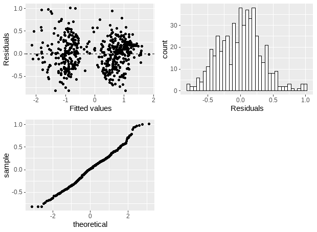
4.2 Machine learning modeling
# Run algorithms using 10-fold cross validation
trainControl <- trainControl(method="repeatedcv", number=10, repeats=3)
metric <- "RMSE"
4.2.1 Evaluate Algorithms: Baseline
# lm
set.seed(7)
fit.lm <- train(audience_score~., data=train_trans, method="lm", metric=metric, trControl=trainControl)
# GLM
set.seed(7)
fit.glm <- train(audience_score~., data=train_trans, method="glm", metric=metric,trControl=trainControl)
# GLMNET
set.seed(7)
fit.glmnet <- train(audience_score~., data=train_trans, method="glmnet", metric=metric,trControl=trainControl)
# SVM
set.seed(7)
fit.svm <- train(audience_score~., data=train_trans, method="svmRadial", metric=metric,trControl=trainControl)
# CART
set.seed(7)
grid <- expand.grid(.cp=c(0, 0.05, 0.1))
fit.cart <- train(audience_score~., data=train_trans, method="rpart", metric=metric,trControl=trainControl)
# KNN
set.seed(7)
fit.knn <- train(audience_score~., data=train_trans, method="knn", metric=metric, trControl=trainControl)
# Compare algorithms
results <- resamples(list(LM=fit.lm, GLM=fit.glm, GLMNET=fit.glmnet, SVM=fit.svm,
                                  CART=fit.cart, KNN=fit.knn))
summary(results)
dotplot(results)
Call:
summary.resamples(object = results)
Models: LM, GLM, GLMNET, SVM, CART, KNN
Number of resamples: 30
MAE
Min. 1st Qu. Median Mean 3rd Qu. Max. NA's
LM 0.2310122 0.2574136 0.2707121 0.2691965 0.2811378 0.3160800 0
GLM 0.2310122 0.2574136 0.2707121 0.2691965 0.2811378 0.3160800 0
GLMNET 0.2310285 0.2507154 0.2657281 0.2667189 0.2803855 0.3135265 0
SVM 0.2502105 0.2889786 0.3066764 0.3063318 0.3253994 0.3615967 0
CART 0.2847380 0.3164592 0.3268184 0.3352146 0.3630442 0.3915826 0
KNN 0.2769875 0.3192514 0.3349857 0.3449373 0.3705548 0.4476559 0
RMSE
Min. 1st Qu. Median Mean 3rd Qu. Max. NA's
LM 0.2985992 0.3177708 0.3337284 0.3392684 0.3545900 0.4078148 0
GLM 0.2985992 0.3177708 0.3337284 0.3392684 0.3545900 0.4078148 0
GLMNET 0.2927227 0.3112989 0.3268975 0.3318891 0.3509410 0.3937352 0
SVM 0.3359649 0.3573947 0.3972685 0.4064684 0.4496446 0.5342493 0
CART 0.3459187 0.3843745 0.4044279 0.4088604 0.4319131 0.4731897 0
KNN 0.3535716 0.3874186 0.4268215 0.4325818 0.4733186 0.5664905 0
Rsquared
Min. 1st Qu. Median Mean 3rd Qu. Max. NA's
LM 0.8476737 0.8785521 0.8876114 0.8884304 0.9003625 0.9281463 0
GLM 0.8476737 0.8785521 0.8876114 0.8884304 0.9003625 0.9281463 0
GLMNET 0.8580913 0.8801078 0.8948029 0.8932897 0.9024593 0.9299116 0
SVM 0.7562335 0.8061196 0.8505634 0.8405477 0.8751151 0.9007095 0
CART 0.8023546 0.8183961 0.8387880 0.8374483 0.8567945 0.8821153 0
KNN 0.7146806 0.7904845 0.8292025 0.8180365 0.8423670 0.8996817 0
4.2.2 Evaluate Algorithms: Feature Selection
# Find and drop attributes that are highly corrected
set.seed(7)
cutoff <- 0.70
correlations <- cor(train_trans[,7:10])
highlyCorrelated <- findCorrelation(correlations, cutoff=cutoff)
for (value in highlyCorrelated) {
  print(names(train_trans[,7:10])[value])
}
[1] "imdb_rating"We can see that we have dropped 1 attributes: imdb_rating.
# create a new dataset without highly corrected features
datasetFeatures <- train_trans[,-highlyCorrelated]
dim(datasetFeatures)
# lm
set.seed(7)
fit.lm <- train(audience_score~., data=datasetFeatures, method="lm", metric=metric, trControl=trainControl)
# GLM Generalized Linear Regression
set.seed(7)
fit.glm <- train(audience_score~., data=datasetFeatures, method="glm", metric=metric,trControl=trainControl)
# GLMNET Penalized Linear Regression
set.seed(7)
fit.glmnet <- train(audience_score~., data=datasetFeatures, method="glmnet", metric=metric,trControl=trainControl)
# SVM
set.seed(7)
fit.svm <- train(audience_score~., data=datasetFeatures, method="svmRadial", metric=metric,trControl=trainControl)
# CART Classification and Regression Trees
set.seed(7)
grid <- expand.grid(.cp=c(0, 0.05, 0.1))
fit.cart <- train(audience_score~., data=datasetFeatures, method="rpart", metric=metric,trControl=trainControl)
# KNN
set.seed(7)
fit.knn <- train(audience_score~., data=datasetFeatures, method="knn", metric=metric, trControl=trainControl)
# Compare algorithms
feature_results <- resamples(list(LM=fit.lm, GLM=fit.glm, GLMNET=fit.glmnet, SVM=fit.svm,
CART=fit.cart, KNN=fit.knn))
summary(feature_results)
dotplot(feature_results)Call:
summary.resamples(object = feature_results)
Models: LM, GLM, GLMNET, SVM, CART, KNN
Number of resamples: 30
MAE
Min. 1st Qu. Median Mean 3rd Qu. Max. NA's
LM 0.2329423 0.2564362 0.2668919 0.2700825 0.2818092 0.3315974 0
GLM 0.2329423 0.2564362 0.2668919 0.2700825 0.2818092 0.3315974 0
GLMNET 0.2284175 0.2526727 0.2649099 0.2669133 0.2815177 0.3163152 0
SVM 0.2249702 0.2625262 0.2743392 0.2765943 0.2932804 0.3404108 0
CART 0.2847380 0.3164592 0.3268184 0.3352146 0.3630442 0.3915826 0
KNN 0.2821982 0.3062210 0.3315394 0.3365520 0.3546523 0.4377836 0
RMSE
Min. 1st Qu. Median Mean 3rd Qu. Max. NA's
LM 0.2954738 0.3133134 0.3297484 0.3376256 0.3512610 0.4119349 0
GLM 0.2954738 0.3133134 0.3297484 0.3376256 0.3512610 0.4119349 0
GLMNET 0.2866947 0.3118496 0.3253406 0.3315956 0.3523885 0.3955532 0
SVM 0.2937697 0.3214932 0.3668399 0.3684543 0.4021538 0.5564881 0
CART 0.3459187 0.3843745 0.4044279 0.4088604 0.4319131 0.4731897 0
KNN 0.3440746 0.3741771 0.4223117 0.4247752 0.4527700 0.5816831 0
Rsquared
Min. 1st Qu. Median Mean 3rd Qu. Max. NA's
LM 0.8429372 0.8764766 0.8898096 0.8892373 0.9016293 0.9261707 0
GLM 0.8429372 0.8764766 0.8898096 0.8892373 0.9016293 0.9261707 0
GLMNET 0.8567947 0.8783813 0.8941842 0.8934166 0.9046634 0.9278666 0
SVM 0.7336090 0.8518095 0.8718849 0.8683236 0.8913415 0.9286218 0
CART 0.8023546 0.8183961 0.8387880 0.8374483 0.8567945 0.8821153 0
KNN 0.6922973 0.8028629 0.8329245 0.8234645 0.8521893 0.9078491 0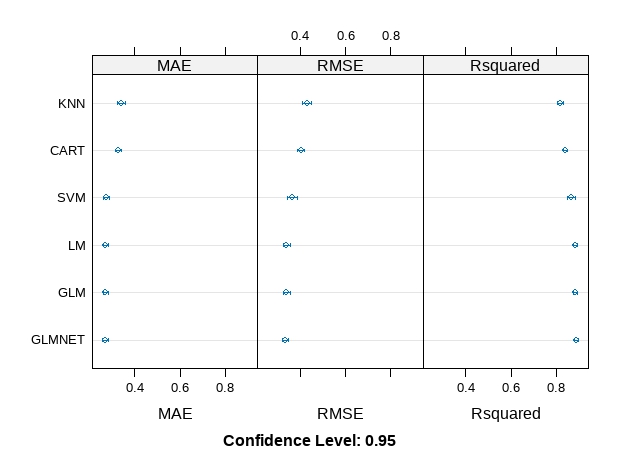
Comparing the results, we can see that this has made the RMSE and Rsquared better for the SVM algorithms, no obvious effect on other models. The correlated attributes we removed are no contributing to the accuracy of other models except SVM. It looks like GLMNET has the lowest RMSE and high Rsquared, followed closely by the other linear algorithms, SVM CART and KNN appear to be in the same ball park and slightly worse error and Rsquared.
4.2.3 Improve Results With Tuning
# Let's look at the default parameters already adopted.
# print(fit.glmnet)
# Make a custom tuning grid.  glmnet is capable of fitting 2 different kinds of penalized models, and it has 2 tuning parameters:
# alpha: Ridge regression (or alpha = 0), Lasso regression (or alpha = 1)
# lambda the strength of the penalty on the coefficients
grid <- expand.grid(alpha = 0:1, lambda = seq(0.0001, 1, length = 10))
# Fit a model
tune.glmnet <- train(audience_score~., data=train_trans, method = "glmnet", metric=metric,
               tuneGrid = grid, trControl = trainControl)
# print(tune.glmnet)
plot(tune.glmnet)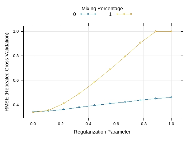
4.2.4 Ensemble Methods
# Random Forest
set.seed(7)
fit.rf <- train(audience_score~., data=train_trans,  method="rf", metric=metric, trControl=trainControl)
# Stochastic Gradient Boosting
set.seed(7)
fit.gbm <- train(audience_score~., data=train_trans,  method="gbm", metric=metric, trControl=trainControl, verbose=FALSE)
# Compare algorithms
ensembleResults <- resamples(list(RF=fit.rf, GBM=fit.gbm))
summary(ensembleResults)
dotplot(ensembleResults)
Call:
summary.resamples(object = ensembleResults)
Models: RF, GBM
Number of resamples: 30
MAE
Min. 1st Qu. Median Mean 3rd Qu. Max. NA's
RF 0.2163944 0.2415927 0.2531496 0.2533204 0.2629469 0.2992215 0
GBM 0.2217354 0.2443042 0.2560293 0.2542399 0.2626921 0.2932200 0
RMSE
Min. 1st Qu. Median Mean 3rd Qu. Max. NA's
RF 0.2832998 0.3143973 0.3227113 0.3284520 0.3452509 0.3905513 0
GBM 0.2783212 0.3112522 0.3186321 0.3249106 0.3382011 0.3807624 0
Rsquared
Min. 1st Qu. Median Mean 3rd Qu. Max. NA's
RF 0.8606755 0.8792828 0.8944804 0.8951121 0.9049159 0.9392259 0
GBM 0.8672786 0.8830680 0.8982563 0.8977297 0.9063247 0.9339450 0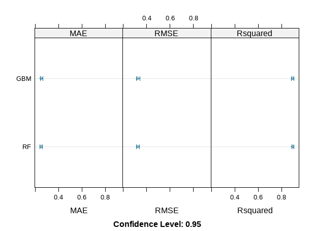
We can see that Gradient Boosting was the most accurate with RMSE and Rsuqared that were better than that achieved by tuning glmnet.
# Improve Results With Tuning
# look at parameters used for Gradient Boosting
# print(fit.gbm)
grid <- expand.grid(interaction.depth = seq(1, 7, by = 2),
                        n.trees = seq(50, 500, by = 50),
                        n.minobsinnode = 10,
                        shrinkage = c(0.01, 0.1))
tune.gbm <- train(audience_score~., data=train_trans,  method="gbm", metric=metric, tuneGrid = grid, trControl=trainControl, verbose=FALSE)
# print(tune.gbm)
plot(tune.gbm)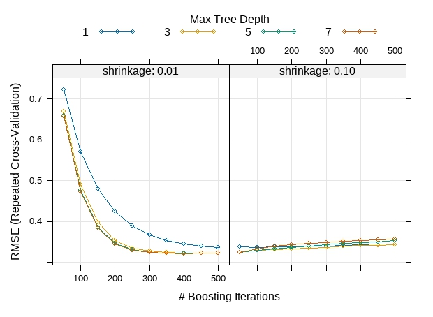
4.2.5 Finalize Model
# train the final model
finalModel <- gbm(audience_score~., data=train_trans, n.trees = 400, interaction.depth = 7, shrinkage = 0.01, n.minobsinnode = 10)
summary(finalModel)
var rel.inf
audience_rating audience_rating 73.24576996
imdb_rating imdb_rating 20.83492961
critics_score critics_score 1.51946427
genre genre 1.44784288
runtime runtime 1.13583662
imdb_num_votes imdb_num_votes 1.05829918
mpaa_rating mpaa_rating 0.62888280
critics_rating critics_rating 0.11715459
title_type title_type 0.01182009
best_pic_win best_pic_win 0.00000000# use final model to make predictions on the testing dataset
# transform testing Data
train$imdb_num_votes <- as.numeric(train$imdb_num_votes)
test_num <- as.data.frame(test[names_n])
# transform the testing dataset using the parameters
transformed_test <- predict(preprocessParams, test_num)
# summarize the transformed dataset
# summary(transformed_test)
test_cat <- as.data.frame(test[names[1:6]])
# combine two datasets in r
test_trans <-cbind(test_cat, transformed_test)
# predictions
predictions <- predict(finalModel, newdata=test_trans)
# calculate RMSE, Rsquared
test_Y <- test_trans[,11]
rmse <- rmse(predictions, test_Y)
#R SQUARED error metric -- Coefficient of Determination
RSQUARE = function(y_actual,y_predict){
cor(y_actual,y_predict)^2
}
r2 <- RSQUARE(test_Y, predictions)
sprintf("RMSE: %#.2f", rmse)
sprintf("R-squared: %#.2f", r2)[1] "RMSE: 0.27"
[1] "R-squared: 0.93"The souce code used to create this blog can be found here.