
1. Introduction
This project involves the analysis of customer usage data for a fitness tracker. Bellabeat, a company that produces FitBit fitness tracker specifically for women. The device can monitor the health vitals of its customers. Bellabeat conduct marketing analytics to expand their business. They have sampled one-month usage data from thirty-three eligible Fitbit users, with their consent. Our task is to gain insights into how existing customers use their products, identify potential trends in Fitbit smart device usage, and leverage these insightful analyses to establish a new market strategy for Bellabeat.
2. Data Preparation
Load Packages and libraries
library(tidyverse)
library(ggplot2)
library(corrplot)
library(gridExtra)
library(naniar) #check nan value
library(lessR) # pie chart
library(NbClust)
library(factoextra)
library(tidyquant)
library(kableExtra)
Load the dataset and take a quick look.
# Check the files locally using Excel and determine which file would be useful.
daily_activity <-read.csv("../FitnessTracker/dailyActivity_merged.csv")
daily_sleep <- read.csv("../FitnessTracker/sleepDay_merged.csv")
weight_log <- read.csv("../FitnessTracker/weightLogInfo_merged.csv")
# Check the number of unique Ids in the dataset
n_distinct(daily_activity$Id)
n_distinct(weight_log$Id)
n_distinct(daily_sleep$Id)
The distinct Id numbers in daily_activity, daily_sleep and weight_log are 33, 24, and 8 respectively. The weight_log dataset may not be useful.
str(daily_activity)'data.frame': 940 obs. of 15 variables:
$ Id : num 1503960366 1503960366 1503960366 1503960366 1503960366 ...
$ ActivityDate : chr "4/12/2016" "4/13/2016" "4/14/2016" "4/15/2016" ...
$ TotalSteps : int 13162 10735 10460 9762 12669 9705 13019 15506 10544 9819 ...
$ TotalDistance : num 8.5 6.97 6.74 6.28 8.16 ...
$ TrackerDistance : num 8.5 6.97 6.74 6.28 8.16 ...
$ LoggedActivitiesDistance: num 0 0 0 0 0 0 0 0 0 0 ...
$ VeryActiveDistance : num 1.88 1.57 2.44 2.14 2.71 ...
$ ModeratelyActiveDistance: num 0.55 0.69 0.4 1.26 0.41 ...
$ LightActiveDistance : num 6.06 4.71 3.91 2.83 5.04 ...
$ SedentaryActiveDistance : num 0 0 0 0 0 0 0 0 0 0 ...
$ VeryActiveMinutes : int 25 21 30 29 36 38 42 50 28 19 ...
$ FairlyActiveMinutes : int 13 19 11 34 10 20 16 31 12 8 ...
$ LightlyActiveMinutes : int 328 217 181 209 221 164 233 264 205 211 ...
$ SedentaryMinutes : int 728 776 1218 726 773 539 1149 775 818 838 ...
$ Calories : int 1985 1797 1776 1745 1863 1728 1921 2035 1786 1775 ...str(daily_sleep)'data.frame': 413 obs. of 5 variables:
$ Id : num 1503960366 1503960366 1503960366 1503960366 1503960366 ...
$ SleepDay : chr "4/12/2016 12:00:00 AM" "4/13/2016 12:00:00 AM" "4/15/2016 12:00:00 AM" "4/16/2016 12:00:00 AM" ...
$ TotalSleepRecords : int 1 2 1 2 1 1 1 1 1 1 ...
$ TotalMinutesAsleep: int 327 384 412 340 700 304 360 325 361 430 ...
$ TotalTimeInBed : int 346 407 442 367 712 320 377 364 384 449 ...Let’s merge and prepare dataset
# Make the date format consistent for daily_activity and data_sleep. For merging/joining dataset easier, we also need to rename both of date column names to the same  .
daily_activity <-daily_activity %>%
  dplyr::rename(date= ActivityDate) %>%
  mutate(date= as_date(date, format= "%m/%d/%Y"))
daily_sleep <- daily_sleep %>%
  dplyr::rename(date= SleepDay) %>%
  mutate(date= as_date(date,format ="%m/%d/%Y %I:%M:%S %p" ))
# Checking the transformed tables
head(daily_activity,2)
glimpse(daily_activity)
head(daily_sleep,2)
glimpse(daily_sleep)
# Let's merge the sleep and activity table using Id and date as reference
merged_daily_activity <- merge(x = daily_activity, y = daily_sleep, by=c("Id","date"), all.x = TRUE)
# Create day of the week feature
merged_daily_activity$day_week <- wday(merged_daily_activity$date, label = TRUE)
# Checking dataset
head(merged_daily_activity,2)
Id date TotalSteps TotalDistance TrackerDistance LoggedActivitiesDistance VeryActiveDistance ModeratelyActiveDistance
1 1503960366 2016-04-12 13162 8.50 8.50 0 1.88 0.55
2 1503960366 2016-04-13 10735 6.97 6.97 0 1.57 0.69
LightActiveDistance SedentaryActiveDistance VeryActiveMinutes FairlyActiveMinutes LightlyActiveMinutes SedentaryMinutes Calories TotalSleepRecords
1 6.06 0 25 13 328 728 1985 1
2 4.71 0 21 19 217 776 1797 2
TotalMinutesAsleep TotalTimeInBed day_week
1 327 346 Tue
2 384 407 WedLet’s check missing values
cat("Number of missing value:", sum(is.na(merged_daily_activity)), "\n")
# plot percentage of missing values per feature
# library(naniar)
gg_miss_var(merged_daily_activity,show_pct=TRUE)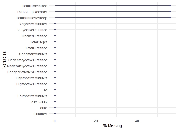
3. EDA
3.1 Correlation between numerical Variable
# Correlation without sleep related data (drop TrackerDistance for redundant with TotalDistance, sleep related columns for not all daily_activity have an equivalent daily_sleep recorded)
data_correlation <- select(merged_daily_activity, TotalSteps:Calories, -TrackerDistance)
corrplot(cor(data_correlation))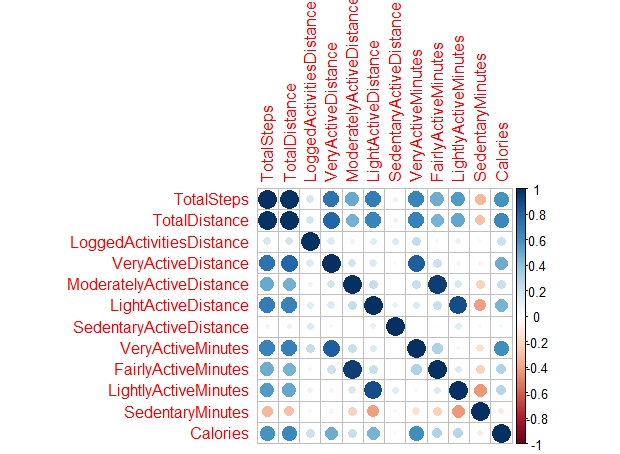
# Correlation with sleep realted data (drop the observations with "NA" on sleep related data)
data_corr_withsleep <- select(merged_daily_activity, TotalSteps:TotalTimeInBed, -TrackerDistance) %>% filter(!is.na(TotalTimeInBed))
corrplot(cor(data_corr_withsleep))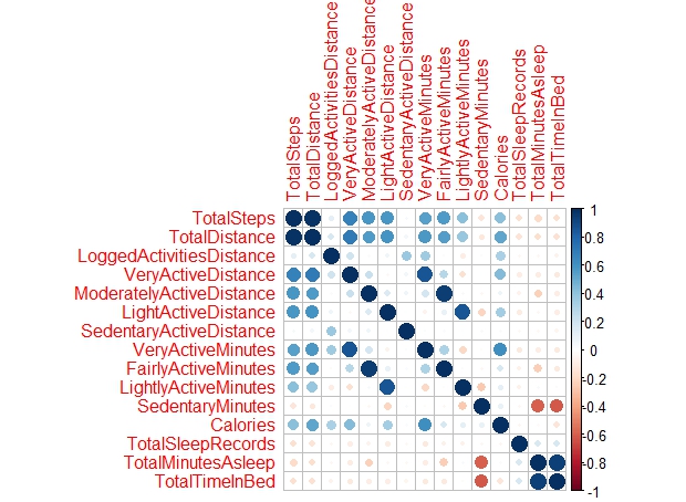
Based on the Correlation Plot, we can see that TotalSteps, TotalDistance (also with high correlation with TotalSteps, collinear), VeryActiveDistance, VeryActiveMinutes, and surprisingly, LightActiveDistance has a high positive correlation with Calories burned. We can summarize that as long as you walk longer distance or greater steps, it won’t matter if it is intense or light activity.
# Relationship of Calories burned with TotalDistance and TotalSteps
names_n <- c("TotalSteps", "VeryActiveDistance", "VeryActiveMinutes", "LightActiveDistance")
plt_list <- list()

for (name in names_n) {
  plt<-ggplot(data = merged_daily_activity, aes_string(x = merged_daily_activity$Calories, y = name)) +
    geom_point(colour = "#33658A") + xlab('Calories')+
    geom_smooth()+
    theme_minimal()
  plt_list[[name]] <- plt
}
plt_grob <- arrangeGrob(grobs=plt_list, ncol=2)
grid.arrange(plt_grob)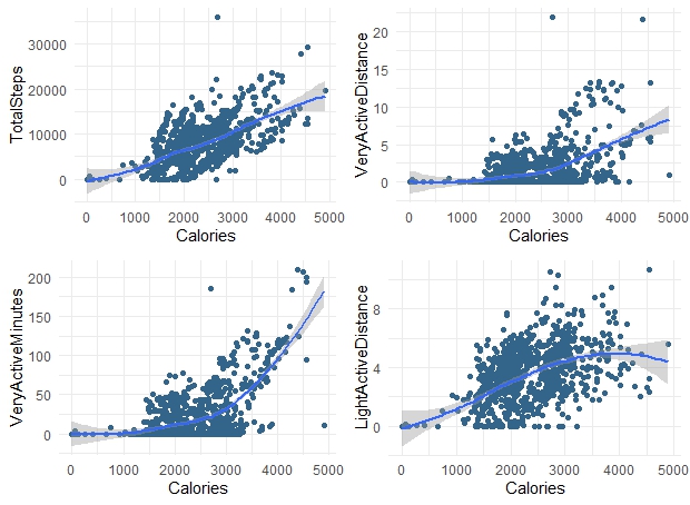
3.2 Analyze tracker Wearing Days by Users
user_usagedays <- merged_daily_activity %>%
  group_by(Id) %>%
  summarise(usagedays = n())
PieChart(usagedays, hole = 0.3, values = "%", data = user_usagedays,main = "Tracker Wearing Days by Users")     # hole = 0 pie chart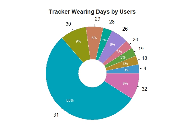
## Data transformation
user <- user_usagedays %>%
  group_by(usagedays) %>% # Variable to be transformed
  count() %>%
  ungroup() %>%
  mutate(perc = n/sum(n)) %>%
  arrange(perc) %>%
  mutate(labels = scales::percent(perc))
user$usagedays<- factor(user$usagedays, levels =user$usagedays)

ggplot(data = user, aes(x = usagedays, y=n)) + geom_bar(stat="identity", fill= "#F6AE2D", colour="black") +
  ylab('Number of users') + xlab('Number of days of wearing') + ggtitle( "Tracker Wearing Days by Users") +
  geom_text(aes(label = n), vjust = 1.5, colour = "black")+
  theme_minimal()     #  "#55DDE0", "#33658A", "#2F4858", "#F6AE2D", "#F26419", "#999999"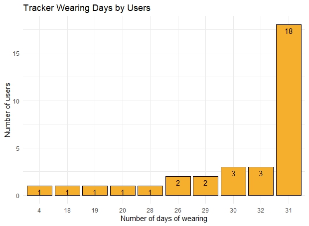
3.3 Analyze user activity behavior by weekday
avg_weekday_activity <- merged_daily_activity %>%
  group_by(day_week) %>%
  summarise_at(c(Avgsteps = "TotalSteps", "Calories", "TotalMinutesAsleep"), mean,na.rm = TRUE) # see how it produces an error because of the "NA" record

names <- names(Filter(is.numeric,avg_weekday_activity))
plt2_list <- list()

for (name in names) {
  plt<-ggplot(data = avg_weekday_activity, aes_string(x= avg_weekday_activity$day_week, y = name, fill = name)) +
    geom_bar(stat="identity") + xlab('Day of Week')+    # geom_bar(stat="identity", fill= "#55DDE0", colour="black")
    scale_fill_gradient (low="light blue", high= "dark blue")+
    theme_minimal()+
    theme(plot.title= element_text(hjust= 0.5,vjust= 0.8, size=16),
                            legend.position= "none")
  plt2_list[[name]] <- plt
}
plt2_grob <- arrangeGrob(grobs=plt2_list, ncol=2)
grid.arrange(plt2_grob)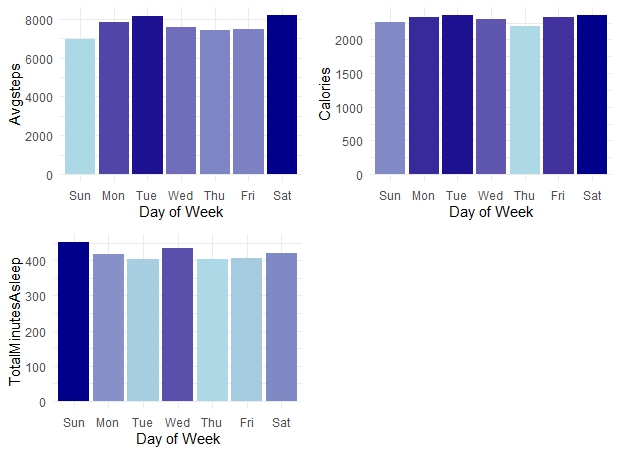
The Activity Plots for the days of the week reveal that our customers were most active on Saturdays, followed closely by Tuesdays. Given that Saturday is a part of the weekend, it’s likely that people had more leisure time to engage in physical activities. Interestingly, Tuesday emerged as the second most active day, a trend that warrants further investigation to understand the underlying cause of this surge in activity. Our data also showed that customers recorded the highest average sleep duration on Sundays, possibly recuperating from the intense activities undertaken on Saturday. Additionally, an increase in sleep observed on Wednesdays aligns with the heightened activity levels seen on Tuesdays
3.4 Analyze user types
3.4.1 Method 1, Based on daily steps, we group users into 4 types: Sedentary, Lightly Active, Fairly Active, and Very Active.
daily_average <- merged_daily_activity %>%
  group_by (Id) %>%
  summarise(avg_daily_steps= mean(TotalSteps),
            avg_daily_cal= mean(Calories),
            avg_daily_sleep= mean(TotalMinutesAsleep,
                                  na.rm = TRUE)) %>%
  mutate(user_type= case_when(
    avg_daily_steps < 5000 ~ "sedentary",
    avg_daily_steps >= 5000 & avg_daily_steps <7499 ~"lightly_active",
    avg_daily_steps >= 7499 & avg_daily_steps <9999 ~"fairly_active",
    avg_daily_steps >= 10000 ~"very_active"
  ))

# summarize life style of users
user_type_sum <- daily_average %>%
  group_by(user_type) %>%
  summarise(user_n= n()) %>%
  mutate(user_perc= user_n/sum(user_n))

ggplot(user_type_sum, aes(x = 1, y = user_perc, fill = user_type)) +
  geom_col(color = "black") +
  geom_text(aes(label = scales::percent(user_perc)), colour = "white", position = position_stack(vjust = 0.5))  +
  coord_polar(theta = "y")+
  guides(fill = guide_legend(title = "Life styles")) +
  scale_fill_viridis_d() +
  theme_void()+    # want a blank slate
  labs(x = NULL, y = NULL, fill = NULL, title = "Life styles by Users")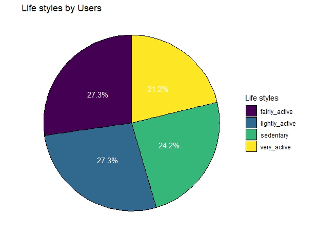
Compare steps, calories, distance & sleep by user type:
p1<-ggplot(daily_average[daily_average[,"avg_daily_steps"] >0, ],
           aes(user_type,avg_daily_steps, fill=user_type))+
  geom_boxplot()+
  stat_summary(fun="mean", geom="point",
               shape=23,size=2, fill="white")+
  labs(title= "Daily Steps by User Type",
       x= " ", y="Steps",
       #caption= 'Data Source: Fitabase Data 4.12.16-5.12.16'
  )+
  scale_fill_brewer(palette="BuPu")+
  theme_minimal()+
  theme(plot.title= element_text(hjust= 0.5,vjust= 0.8, size=12),axis.text.x = element_text(angle = 15, vjust = 1.5, hjust=0.5),
        legend.position= "none")

p2<-ggplot(daily_average[daily_average[,"avg_daily_cal"] >0, ],
           aes(user_type,avg_daily_cal, fill=user_type))+
  geom_boxplot()+
  stat_summary(fun="mean", geom="point",
               shape=23,size=2, fill="white")+
  labs(title= "Daily Burned Calories by User Type",
       x= " ", y="Calories",
       #caption= 'Data Source: Fitabase Data 4.12.16-5.12.16'
  )+
  scale_fill_brewer(palette="BuPu")+
  theme_minimal()+
  theme(plot.title= element_text(hjust= 0.5,vjust= 0.8, size=12),axis.text.x = element_text(angle = 15, vjust = 1.5, hjust=0.5),
        legend.position= "none")

p3<-ggplot(na.omit(daily_average[daily_average[,"avg_daily_sleep"] >0, ]),
           aes(user_type,avg_daily_sleep, fill=user_type))+
  geom_boxplot()+
  stat_summary(fun="mean", geom="point",
               shape=23,size=2, fill="white")+
  labs(title= " Daily Asleep by User Type",
       x= " ", y="Minutes Asleep",
       #caption= 'Data Source: Fitabase Data 4.12.16-5.12.16'
  )+
  scale_fill_brewer(palette="BuPu")+
  theme_minimal()+
  theme(plot.title= element_text(hjust= 0.5,vjust= 0.8, size=12),axis.text.x = element_text(angle = 15, vjust = 1.5, hjust=0.5),
        legend.position= "none")
grid.arrange(p1,p2,p3,ncol=2)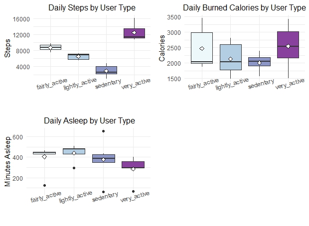
3.4.2 Method 2: use clustering method to segment users
user_average <- merged_daily_activity %>%
  group_by(Id) %>%
  summarise_at(c(2:17),mean,na.rm = TRUE) %>%
  rename_with(~str_replace(., 'Total', 'Avg'))  %>%
  mutate(Id = as.character(Id))
# corrplot(cor(select(user_average, AvgSteps:Calories, -TrackerDistance)))
# Scale the data
user_average_scaled <- scale(select(user_average, AvgSteps,VeryActiveMinutes:Calories))
# Determine how many clusters we can make
nb <- NbClust(user_average_scaled, distance = "euclidean", min.nc = 2,
              max.nc = 6, method = "kmeans")
#fviz_nbclust(nb)
# Three is the best cluster number. We will use 3 clusters to group these users for simplicity
km_res <- kmeans(user_average_scaled, centers = 3, nstart = 35)
fviz_cluster(km_res, geom = "point", data=user_average_scaled,ggtheme = theme_minimal())+ggtitle("k-means clustering K=3")
# Lets also check the amount of customers in each cluster.
km_res$size
# centroids from model on normalized data
km_res$centers 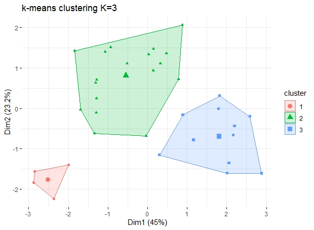
Analysis clustering results
# add cluster into user_average dataset
user_average <- user_average %>%
  mutate(Cluster = km_res$cluster)

user_average <- user_average %>%
  mutate(Segment = ifelse(Cluster == 1, "Very Active",
                          ifelse(Cluster == 2, "Lightly Active", "Sedentary")))

user_K3 <- user_average %>% select(Segment, AvgSteps,VeryActiveMinutes:Calories)%>% group_by(Segment) %>% summarise_all("mean") %>%
  ungroup() %>% kable() %>% kable_styling()
user_K3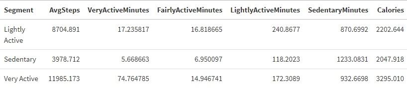
compare by users
user2_type_sum <- user_average %>%
  group_by(Segment) %>%
  summarise(user_n= n()) %>%
  mutate(user_perc= user_n/sum(user_n))%>%
  arrange(user_perc)

ggplot(user2_type_sum, aes(x = 1, y = user_perc, fill = Segment)) +
  geom_col(color = "black") +
  geom_text(aes(label =scales::percent(user_perc)), colour = "white",  position = position_stack(vjust = 0.5))  +
  coord_polar(theta = "y", start=0)+
  guides(fill = guide_legend(title = "Life styles")) +
  scale_fill_viridis_d() +
  theme_void()+    # want a blank slate
  labs(x = NULL, y = NULL, fill = NULL, title = "Life styles by Users -- Kmean")


p1<-ggplot(user_average[user_average[,"AvgSteps"] >0, ],    #group_daily_activity[which(group_daily_activity$TotalSteps>0),]
           aes(Segment,AvgSteps, fill=Segment))+
  geom_boxplot()+
  stat_summary(fun="mean", geom="point",
               shape=23,size=2, fill="white")+
  labs(title= "Daily Steps by User Type",
       x= " ", y="Steps",
       #caption= 'Data Source: Fitabase Data 4.12.16-5.12.16'
  )+
  scale_fill_brewer(palette="BuPu")+
  theme_minimal()+
  theme(plot.title= element_text(hjust= 0.5,vjust= 0.8, size=16),axis.text.x = element_text(angle = 15, vjust = 1.5, hjust=0.5),
        legend.position= "none")


p2<-ggplot(user_average[user_average[,"Calories"] >0, ],    #group_daily_activity[which(group_daily_activity$TotalSteps>0),]
           aes(Segment,Calories, fill=Segment))+
  geom_boxplot()+
  stat_summary(fun="mean", geom="point",
               shape=23,size=2, fill="white")+
  labs(title= "Daily Burned Calories by User Type",
       x= " ", y="Calories",
       #caption= 'Data Source: Fitabase Data 4.12.16-5.12.16'
  )+
  scale_fill_brewer(palette="BuPu")+
  theme_minimal()+
  theme(plot.title= element_text(hjust= 0.5,vjust= 0.8, size=16),axis.text.x = element_text(angle = 15, vjust = 1.5, hjust=0.5),
        legend.position= "none")

p3<-ggplot(na.omit(user_average[user_average[,"AvgMinutesAsleep"] >0, ]),    #group_daily_activity[which(group_daily_activity$TotalSteps>0),]
           aes(Segment,AvgMinutesAsleep, fill=Segment))+
  geom_boxplot()+
  stat_summary(fun="mean", geom="point",
               shape=23,size=2, fill="white")+
  labs(title= " Daily Asleep by User Type",
       x= " ", y="Minutes Asleep",
       #caption= 'Data Source: Fitabase Data 4.12.16-5.12.16'
  )+
  scale_fill_brewer(palette="BuPu")+
  theme_minimal()+
  theme(plot.title= element_text(hjust= 0.5,vjust= 0.8, size=16),axis.text.x = element_text(angle = 15, vjust = 1.5, hjust=0.5),
        legend.position= "none")
grid.arrange(p1,p2,p3,ncol=2)

p4<-ggplot(user_average[user_average[,"VeryActiveMinutes"] >0, ],    #group_daily_activity[which(group_daily_activity$TotalSteps>0),]
           aes(Segment,VeryActiveMinutes, fill=Segment))+
  geom_boxplot()+
  stat_summary(fun="mean", geom="point",
               shape=23,size=2, fill="white")+
  labs(title= "Very Active Minutes  by User Type",
       x= " ", y="VeryActiveMinutes ",
       #caption= 'Data Source: Fitabase Data 4.12.16-5.12.16'
  )+
  scale_fill_brewer(palette="BuPu")+
  theme_minimal()+
  theme(plot.title= element_text(hjust= 0.5,vjust= 0.8, size=16),axis.text.x = element_text(angle = 15, vjust = 1.5, hjust=0.5),
        legend.position= "none")


p5<-ggplot(user_average[user_average[,"FairlyActiveMinutes"] >0, ],    #group_daily_activity[which(group_daily_activity$TotalSteps>0),]
           aes(Segment,FairlyActiveMinutes, fill=Segment))+
  geom_boxplot()+
  stat_summary(fun="mean", geom="point",
               shape=23,size=2, fill="white")+
  labs(title= "Fairly Active Minutes by User Type",
       x= " ", y="Fairly Active Minutes ",
       #caption= 'Data Source: Fitabase Data 4.12.16-5.12.16'
  )+
  scale_fill_brewer(palette="BuPu")+
  theme_minimal()+
  theme(plot.title= element_text(hjust= 0.5,vjust= 0.8, size=16),axis.text.x = element_text(angle = 15, vjust = 1.5, hjust=0.5),
        legend.position= "none")

p6<-ggplot(user_average[user_average[,"LightlyActiveMinutes"] >0, ],    #group_daily_activity[which(group_daily_activity$TotalSteps>0),]
           aes(Segment,LightlyActiveMinutes, fill=Segment))+
  geom_boxplot()+
  stat_summary(fun="mean", geom="point",
               shape=23,size=2, fill="white")+
  labs(title= "Lightly Active Minutes by User Type",
       x= " ", y="Lightly Active Minutes ",
       #caption= 'Data Source: Fitabase Data 4.12.16-5.12.16'
  )+
  scale_fill_brewer(palette="BuPu")+
  theme_minimal()+
  theme(plot.title= element_text(hjust= 0.5,vjust= 0.8, size=16),axis.text.x = element_text(angle = 15, vjust = 1.5, hjust=0.5),
        legend.position= "none")

p7<-ggplot(na.omit(user_average[user_average[,"SedentaryMinutes"] >0, ]),    #group_daily_activity[which(group_daily_activity$TotalSteps>0),]
           aes(Segment,SedentaryMinutes, fill=Segment))+
  geom_boxplot()+
  stat_summary(fun="mean", geom="point",
               shape=23,size=2, fill="white")+
  labs(title= "Sedentary Minutes by User Type",
       x= " ", y="Sedentary Minutes   ",
       #caption= 'Data Source: Fitabase Data 4.12.16-5.12.16'
  )+
  scale_fill_brewer(palette="BuPu")+
  theme_minimal()+
  theme(plot.title= element_text(hjust= 0.5,vjust= 0.8, size=16),axis.text.x = element_text(angle = 15, vjust = 1.5, hjust=0.5),
        legend.position= "none")
grid.arrange(p4,p5,p6,p7, ncol=2)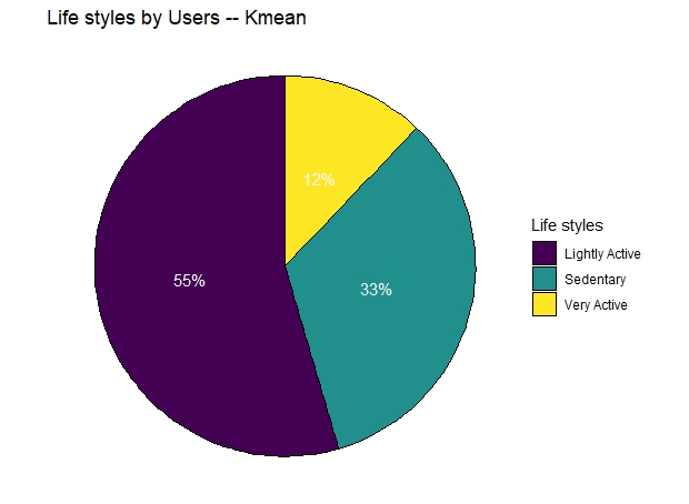
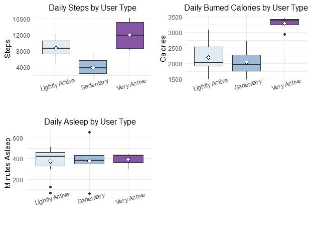
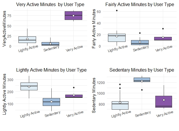
Utilizing the k-means clustering method, we have segmented all users into three distinct groups: very active, lightly active, and sedentary. The ‘very active’ users, typically sports enthusiasts, constitute approximately 12% of all users. They exhibit high-intensity exercise, as evidenced by their daily average steps, intense exercise duration, and calories burned, which significantly surpass those of the other two groups. The ‘lightly active’ users make up 55% of the total user base. Although their daily average steps exceed those of the sedentary group, their daily average calories burned show no significant difference. This is likely due to insufficient high-intensity activity. Extended periods of sedentary behavior are the primary reason users are categorized as ‘sedentary’. We also can get a result from above analysis that high intense exercise duration is the best way for burning calories, but if you just wonder to advoid a sedentary lifestyle, you need to reduce longtime sitting and engage in any active activities to increase step count and distance.
3.5 Analyze Heart Rate
heartrate <- read.csv("../FitnessTracker/heartrate_seconds_merged.csv")
# check data structure
str(heartrate)
# Summary Statistics
summary(heartrate)
ggplot(data = heartrate, aes(x = Value)) +
  geom_histogram(aes(y=100*(..count..)/sum(..count..)), color='black', fill="#55DDE0") + ylab('percentage') +
  ggtitle("Heartrate Histogram")+
theme_minimal() 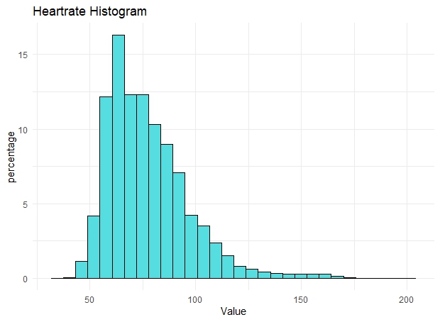
The histogram shows some extreme values for heart rate, with over 200 beats per minute (BPM), which is very dangerous even on an intense activity. Let’s check those record with more than 200 BPM.
3.5.1 Find anomaly value
heartrate <- heartrate %>%
  mutate(Time = mdy_hms(Time), Weekday=weekdays(Time), Hour= format(Time, format = "%H"), Date= format(Time, format = "%m-%d-%y"))
heartrate_anomaly <- heartrate %>% filter(Value >= 200)
heartrate_anomaly
distinct(heartrate %>% filter(Value >= 200), Id)
Id Time Value Weekday Hour Date
1 2022484408 2016-04-21 16:31:20 200 Thursday 16 04-21-16
2 2022484408 2016-04-21 16:31:30 202 Thursday 16 04-21-16
3 2022484408 2016-04-21 16:31:40 203 Thursday 16 04-21-16
4 2022484408 2016-04-21 16:31:50 202 Thursday 16 04-21-16
5 2022484408 2016-04-21 16:32:00 203 Thursday 16 04-21-16
6 2022484408 2016-04-21 16:32:10 203 Thursday 16 04-21-16
7 2022484408 2016-04-21 16:32:20 203 Thursday 16 04-21-16
8 2022484408 2016-04-21 16:32:35 203 Thursday 16 04-21-16
9 2022484408 2016-04-21 16:32:40 201 Thursday 16 04-21-16
10 2022484408 2016-04-21 16:32:50 200 Thursday 16 04-21-16
11 2022484408 2016-04-21 16:33:05 200 Thursday 16 04-21-16
12 2022484408 2016-04-21 17:05:40 202 Thursday 17 04-21-16
13 2022484408 2016-04-21 17:05:50 203 Thursday 17 04-21-16
14 2022484408 2016-04-21 17:06:05 203 Thursday 17 04-21-16
15 2022484408 2016-04-21 17:06:20 203 Thursday 17 04-21-16
16 2022484408 2016-04-21 17:06:30 202 Thursday 17 04-21-16
17 2022484408 2016-04-21 17:06:40 200 Thursday 17 04-21-16
Id
1 2022484408heartrate_p2 <- heartrate[heartrate$Id==2022484408 & heartrate$Date=="04-21-16",]
ggplot(heartrate_p2, aes(x=Time, y=Value)) +
geom_line(color = 'darkgreen') +
geom_hline(aes(yintercept=200), colour="#990000", linetype="dashed") + #This is our control line
geom_text(x=strptime("2016-04-21 07:30:00", "%Y-%m-%d %H:%M:%S"), y=204, label="Heart Rate = 200") +
geom_text(x=strptime("2016-04-21 12:00:00", "%Y-%m-%d %H:%M:%S"), y=100, label="1 hour SMA Line") +
geom_ma(ma_fun = SMA, n = 720, color = 'blue', size = 5) + # plot 1 hour moving average line
theme(axis.text.x = element_text(angle = 0, vjust = 1.0, hjust = 1.0)) +
labs(title= "Heart Rate Of User ID = 2022484408 in April 12th",
y="Heart Rate BPM",
)+
theme_minimal() 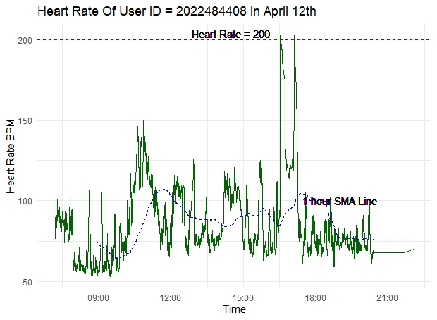
3.5.2 Compare average heart rate by user type
heartrate_avg <- heartrate %>%
  group_by(Id) %>%
  summarise(Avgheartrate = mean(Value)) %>%
  ungroup()

merged_heartrate <- merge(heartrate_avg, user_average[c("Id","Segment")], by="Id", all.x = TRUE)

ggplot(merged_heartrate,aes(Segment,Avgheartrate, fill=Segment))+
  geom_boxplot()+
  stat_summary(fun="mean", geom="point",
               shape=23,size=2, fill="white")+
  labs(title= "Average Heart Rate by User Type",
       x= " ", y="Heart Rate",
       #caption= 'Data Source: Fitabase Data 4.12.16-5.12.16'
  )+
  scale_fill_brewer(palette="BuPu")+
  theme_minimal()+
  theme(plot.title= element_text(hjust= 0.5,vjust= 0.8, size=16),axis.text.x = element_text(angle = 15, vjust = 1.5, hjust=0.5),
        legend.position= "none")
4. Product Marketing Strategy
A fitness tracker can be a valuable tool for health enthusiasts, as it monitors user activity to promote a healthier lifestyle. Our new marketing strategy for this device emphasizes its professional fitness and health features.
-
Customized Exercise Regimen by User Type
We can offer a range of exercise regimens tailored to different user types. By providing the lower, upper quartiles, and average steps, distance, and calories burned for each user type, customers can strive for a healthier lifestyle by challenging themselves with more high-intensity exercises or maintaining an exercise routine that aligns with their preferred lifestyle.
-
Tools to Enhance Exercise Motivation
Our activity trend graph reveals that exercise varies throughout the week, with Saturday and Tuesday being the most active days. We recommend customers to set higher intensity exercise goals on these days. Users can also designate their own ‘warrior’ days to challenge themselves with more vigorous exercises. Notifications about local sports events or club activities, or the connection with exercise social platforms, could significantly motivate users to increase their physical activity.
-
Enhanced Health Alert Features
As a fitness device, it’s crucial to include an alert function for abnormal health vital signs, such as sudden increases or decrease exceeding normal range in BPM, oxygen level and blood pressure. A feature where the device can contact an emergency hotline or a designated person in case of emergency would be a valuable addition. Reminders promoting a healthy lifestyle are also essential, such as movement reminders after prolonged sedentary periods, late sleep reminders, and alerts for significantly reduced sleep time.
The souce code used to create this blog can be found here.